Tutorial 2. Selecting the biogeographic model

Summary:

This tutorial describes the use of RASP to analyze the Hawaiian Psychotria (Nepokroeff et al., 2003) data as in Ree and Smith (2008). It will take you through the process of importing phylogenetic trees, making choices about the model and inferring biogeographic history.

All files used in this tutorial are stored in examples/Psychotria/. If you are a beginner of RASP, please start from Tutorial 1.  

Loading the data files

Open [File > Load Trees> Load Trees (more format)] and navigate to Trees_States /dataset.trees and select it.

Open [File> Load Consensus Tree> Load User-specified Tree] and navigate to Trees_States/Psychotria.tree and select it.

Open [File > Load States (Distributions)], navigate to Trees_States/distribution.csv and select it.

Selecting the biogeographic model

In RASP, we use the R package ‘BioGeoBEARS’ (Matzke 2014) to select the historical biogeography model.

Open [Reconstruction> Model Test> Compare Six Models Using BioGeoBEARS], you will see a window like this:

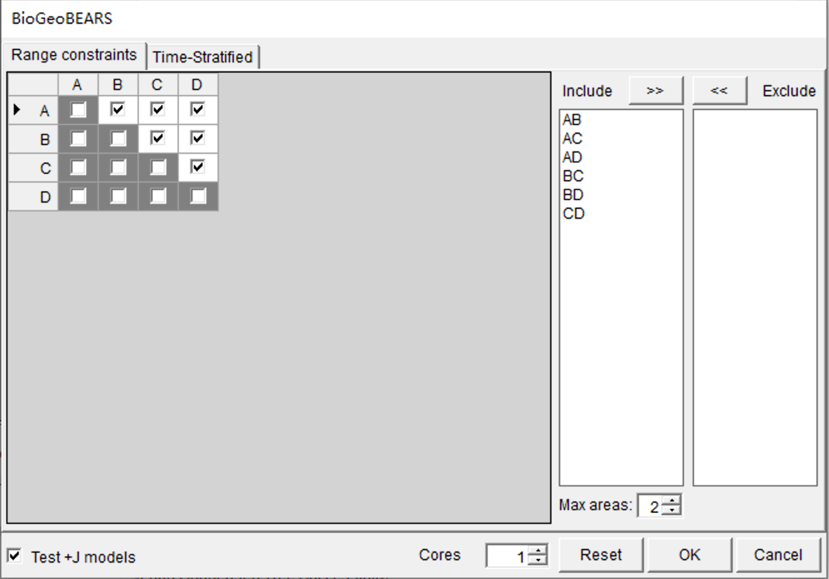
Keep everything as default and click OK. The “Cores” option can be used to increase the speed of analyses that are more computationally intensive. The “Max areas” defines the number of unit areas allowed in ancestral distributions. The list of “Include” will be updated when you change the value of “Max areas” (See 3.3.1 in Manual of RASP for the details of settings).

NOTE: Since the +J models implemented in BGB have been criticized by Ree and Sanmartín (2018), we leave the choice to the reader to decide whether to test/use the +J model or not (Test +J models option).

NOTE: Variation in dispersal can be specified by time periods in which particular constraints can be enforced. If you want to repeat the analyses of Ree and Smith (2008), you also need to load a time‐stratification file under the Time-Stratified tab. Click [Import] button in Time-Stratified tab, navigate to

examples/Psychotria/States/timeperiods.txt and select it.

You may see a command window (in Windows) with some text. Keep it open until it closes automatically. This took 30 seconds to run on a 3.0 GHz CPU laptop.

NOTE: Users will see a lot of information presented in the bottom of the RASP window, including relevant citations, the results of model testing and some suggestions. The analysis log can be saved using [File> Save> Save Logs]

Open [Graphic> Tree View] and you will see a window like the following:

The list to the left shows the inferred biogeographic history on the consensus tree with different models. To select the best fit model, click the Supplement tab to see the details of the model test. Results can be saved using [File> Save Info> Supplement Information] in this window and then opened in Excel. See Results/model_test.xls.

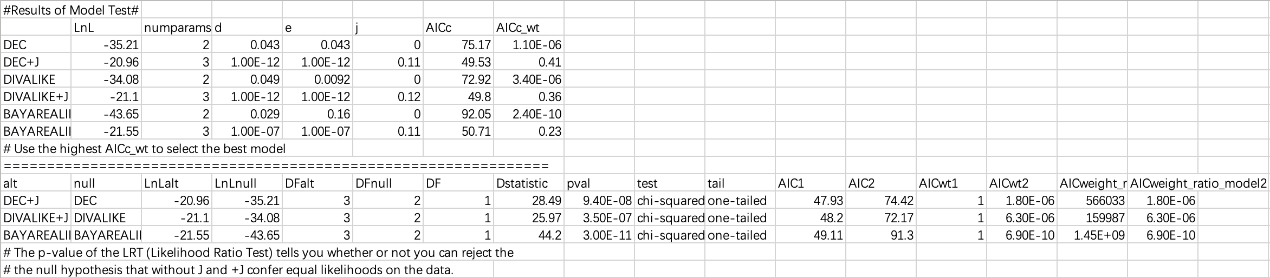
You could simply choose the model with the highest AICc_wt value as the 'Best' model. In the above result, we can see that DEC+J has the highest AICc_wt value of 0.41. We will use this model in the subsequent analysis

NOTE: The p-value of the LRT (Likelihood Ratio Test) tells you whether or not you can reject the null hypothesis that -J and +J confer equal likelihoods on the data.

Apply the model on trees dataset

Usually, the trees dataset contains hundreds or thousands of trees. We can randomly subsample trees to decrease the calculation time. By default, RASP will select 100 trees from the trees file. You can change the default values in the upper right of main window.

NOTE: Users can define a seed for the random method in [Tools> Seed For Random Trees]

Open [Reconstruction> On Trees> Statistical DIVALIKE/DEC/BAYAREALIKE in BioGeoBEARS (S-BGB)], you will see a window like this:

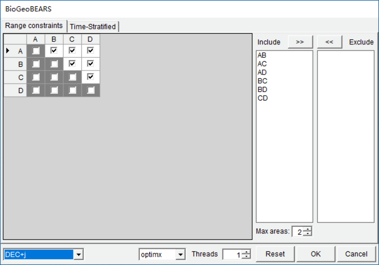
Select “DEC+J” model in the selection box at the left bottom. This took about 5 minutes to run on a 3.0 GHz CPU with default settings. Open [Graphic->Tree View] to see the results.

NOTE: Users can set a larger value for “Threads” to speed up the analysis if you have a multicore CPU.

References

Nepokroeff, M., Sytsma, K. J., Wagner, W. L., & Zimmer, E. A. (2003). Reconstructing Ancestral Patterns of Colonization and Dispersal in the Hawaiian Understory Tree Genus Psychotria (Rubiaceae); A Comparison of Parsimony and Likelihood Approaches. Systematic Biology, 52(6), 820-838

Ree, R. H. & Smith, S. A. (2008). Maximum likelihood inference of geographic range evolution by dispersal, local extinction, and cladogenesis. Systematic Biology, 57(1), 4-14.

Ree, R. H. & Sanmartín, I. (2018). Conceptual and statistical problems with the DEC+ J model of founder‐event speciation and its comparison with DEC via model selection. Journal of Biogeography, 45(4), 741-749.

Matzke, N. J. (2014). Model selection in historical biogeography reveals that founder-event speciation is a crucial process in island clades. Systematic Biology, 63(6), 951-970.